Basic Layers

Apart from the basic nodes we encountered in the previous chapter, PyTorch also provides us with more complex layers that encapsulate groups of nodes. From the perspective of the computational graph, a layer is basically a subgraph of the computational graph.

However, it is usually more helpful to treat layers as mathematical functions that take input tensors and produce output tensors.

Layers are located in the torch.nn package, so we need to import it along with a few other packages:

import numpy as np
import matplotlib.pyplot as plt
import torch
import torch.nn as nn
import torch.optim as optim

We will also set the seed for generating random numbers to improve reproducibility of our examples:

torch.manual_seed(42)

<torch._C.Generator at 0x7fd53c6c3d70>

We will also disable scientific mode for printing to simplify how our tensors are output to the console:

torch.set_printoptions(sci_mode=False)

The Linear Layer

One of the simplest and most important layers is the linear layer.

The linear layer represents the function \(f(\vec{x}) = W\vec{x} + \vec{b}\). Put differently, the linear layer takes an input tensor \(\vec{x}\) and produces an output tensor \(\vec{y} = W\vec{x} + \vec{b}\).

Usually, the matrix W is referred to as the weight matrix, and the vector b as the bias.

When thinking about a layer, it helps to consider the dimensions of the tensors involved. Let’s look at an example where \(\vec{x}\) has \(3\) features, i.e. \(\vec{x} \in \mathbb{R}^{3}\). Let \(\vec{y}\) represent a probability distribution over \(4\) classes, i.e. \(\vec{y} \in \mathbb{R}^{4}\). Then, we have \(W \in \mathbb{R}^{4 \times 3}\) and \(\vec{b} \in \mathbb{R}^{4}\) (otherwise, the dimensions won’t match).

This is how the above example would look in code:

d_in = 3
d_out = 4

x = torch.randn(d_in)

layer = nn.Linear(in_features=d_in, out_features=d_out)

y = layer(x)

Observe how the usage of the layer further emphasizes its nature as a mathematical function. Indeed, the layer can be called as a function that takes an input argument x and simply produces an output argument y.

Let’s now verify that the dimensions and values are what we expect.

First, let’s check that x is a one-dimensional tensor (i.e. a vector) of size 3:

print(x)

tensor([0.3367, 0.1288, 0.2345])

print(x.size())

torch.Size([3])

Next, let’s verify that y is a one-dimensional tensor (i.e. a vector) of size 4:

print(y)

tensor([-0.0315,  0.0420, -0.0469,  0.4115], grad_fn=<ViewBackward0>)

print(y.size())

torch.Size([4])

Next, let’s verify that W is a two-dimensional tensor (i.e. a matrix) of size 4x3:

print(layer.weight)

Parameter containing:
tensor([[ 0.5090, -0.4236,  0.5018],
        [ 0.1081,  0.4266,  0.0782],
        [ 0.2784, -0.0815,  0.4451],
        [ 0.0853, -0.2695,  0.1472]], requires_grad=True)

print(layer.weight.shape)

torch.Size([4, 3])

And finally, we check that b is a one-dimensional tensor (i.e. a vector) of size 4:

print(layer.bias)

Parameter containing:
tensor([-0.2660, -0.0677, -0.2345,  0.3830], requires_grad=True)

print(layer.bias.shape)

torch.Size([4])

Put more generally, if we have an input vector \(\vec{x} \in \mathbb{R}^d\), the linear layer with parameters \(W \in \mathbb{R}^{k \times d}\) and \(\vec{b} \in \mathbb{R}^k\) will compute an output vector \(\vec{y} \in \mathbb{R}^k\). Always keep thinking about tensor dimensionalities - this is really helpful when you are trying to understand a layer.

Let’s also check that the linear layer indeed performs the calculation \(f(\vec{x}) = W\vec{x} + \vec{b}\):

manual_y = torch.matmul(layer.weight, x) + layer.bias

print(manual_y)

tensor([-0.0315,  0.0420, -0.0469,  0.4115], grad_fn=<AddBackward0>)

print((y == manual_y).all())

tensor(True)

Redoing the calculations of a layer manually is not something you will do in production, but it’s a great way to ensure that your understanding is correct.

Note that we can pass a batch through the linear layer:

batch_dim = 2

X = torch.randn(batch_dim, d_in)
Y = layer(X)

print(X.shape)

torch.Size([2, 3])

print(Y.shape)

torch.Size([2, 4])

Compared to the vectors x and y from before, the tensors X and Y now have an additional dimension - the batch dimension. Basically, we can compute the linear layer for multiple vectors at the same time, which greatly speeds up the computation.

We can verify that Y contains the result of applying the linear function \(f(\vec{x}) = W\vec{x} + \vec{b}\) to every row of X at the same time:

manual_y_0 = torch.matmul(layer.weight, X[0]) + layer.bias
manual_y_1 = torch.matmul(layer.weight, X[1]) + layer.bias
manual_Y = torch.stack((manual_y_0, manual_y_1), dim=0)

print(Y)

tensor([[    -1.4670,      0.2987,     -1.0130,     -0.1453],
        [    -0.5116,      0.3374,      0.0005,      0.2350]],
       grad_fn=<AddmmBackward0>)

print(manual_Y)

tensor([[    -1.4670,      0.2987,     -1.0130,     -0.1453],
        [    -0.5116,      0.3374,      0.0005,      0.2350]],
       grad_fn=<StackBackward0>)

print((Y == manual_Y).all())

tensor(True)

As discussed in the chapter on computational graphs, when we train a neural network we really update its parameters. Now, that we have layers, we update the parameters of the layers. In the case of the linear layer, these are W and b.

We can view all learnable parameters of a layer using the parameters() and named_parameters() methods:

for param in layer.parameters():
    print(param)

Parameter containing:
tensor([[ 0.5090, -0.4236,  0.5018],
        [ 0.1081,  0.4266,  0.0782],
        [ 0.2784, -0.0815,  0.4451],
        [ 0.0853, -0.2695,  0.1472]], requires_grad=True)
Parameter containing:
tensor([-0.2660, -0.0677, -0.2345,  0.3830], requires_grad=True)

for name, param in layer.named_parameters():
    print(name, param)

weight Parameter containing:
tensor([[ 0.5090, -0.4236,  0.5018],
        [ 0.1081,  0.4266,  0.0782],
        [ 0.2784, -0.0815,  0.4451],
        [ 0.0853, -0.2695,  0.1472]], requires_grad=True)
bias Parameter containing:
tensor([-0.2660, -0.0677, -0.2345,  0.3830], requires_grad=True)

Activation Functions

So far our learning hasn’t been really deep, which is kind of a shame given that the field this book is about is called deep learning.

Instead of having a single layer, with modern neural networks, we have multiple layers on top of each other. The idea here is that each layer learns progressively more complex features. For example, the first layer might learn how individual words interact with each other, the second layer might look at word groups and the third layer might look at sentences. Note that this is just an example - in practice, the layers learn much more complicated features that can’t be easily described (this is also one of their drawbacks).

How would we go about constructing such a deep network?

Unfortunately, we can’t just put linear layers on top of each other. Consider two linear layers that compute \(\vec{h} = W\vec{x} + \vec{b}\) and \(\vec{y} = V\vec{h} + \vec{c}\) respectively. Then, we would have \(\vec{y} = V\vec{h} + \vec{c} = V(W\vec{x} + \vec{b} + \vec{c}) = VW\vec{x} + V\vec{b} + \vec{c}\). Let \(U = VW\) and \(\vec{d} = V\vec{b} + \vec{c}\), and we can see that \(\vec{y} = U\vec{x} + \vec{c}\). Therefore, the composition of two linear layers is again a linear layer!

If you know your linear algebra, the above computation was a trivial exercise, but it reveals an important truth. We need to go beyond linearities to obtain models with rich capabilities.

To solve this problem, we introduce a nonlinear activation function between the layers to break the linearity. That is, the first layer computes \(\vec{h} = f(W\vec{x} + \vec{b})\), where \(f\) is some nonlinear function and is usually applied elementwise to the vector \(W\vec{x} + \vec{b}\).

If we have two linear layers separated by a nonlinear activation function, the resulting function is no longer linear, and we can build impressively capable models. With the idea clear, we need to actually define the activation function.

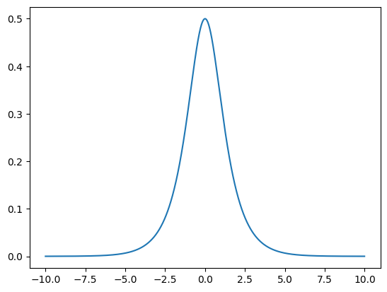
We could use the sigmoid from the chapter on computational graphs. However, this function has a problem that becomes evident when we examine the graph of its derivative:

sigmoid_derivative_xs = np.arange(-10, 10, 0.01)
sigmoid_derivative_ys = np.exp(-sigmoid_derivative_xs) / (1 + np.exp(-sigmoid_derivative_xs) ** 2)
plt.plot(sigmoid_derivative_xs, sigmoid_derivative_ys)

[<matplotlib.lines.Line2D at 0x7fd48cf0aac0>]

The derivative of the sigmoid function is very close to \(0\) outside a relatively small input range. Why is this a problem?

Let’s say that during backpropagation the sigmoid node receives a derivative \(\frac{\partial L}{\partial y}\) (where \(y\) is the output of the sigmoid node). It will then backpropagate the derivative \(\frac{\partial L}{\partial z} = \frac{\partial L}{\partial y} \frac{\partial y}{\partial z}\). But if \(\frac{\partial y}{\partial z}\) is approximately \(0\), the derivative \(\frac{\partial L}{\partial z}\) will be approximately \(0\) as well. The derivative (and therefore, the error signal) is now lost.

Just as a side note, the above explanation is an example of why it is so important to actually understand what backpropagation does on a technical level even though you will probably never need to implement it. It would be very hard to grasp why sigmoids are a bad idea for activation functions unless you are actually capable of doing the math (luckily the math to do is really not that complicated). This is not the last time we will encounter a problem that has its roots in the way backpropagation operates.

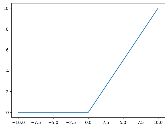
Executive summary - we need a different activation function that doesn’t have such a small “good” range of inputs. A very simple way to address this is to take the identity function and cut off half the input range resulting in \(f(x) = \max(0, x)\):

relu_xs = np.arange(-10, 10, 0.01)
relu_ys = np.maximum(0, relu_xs)
plt.plot(relu_xs, relu_ys)

[<matplotlib.lines.Line2D at 0x7fd48ae09d30>]

The derivative of this function is \(0\) if \(x < 0\) and \(1\) if \(x > 0\) (we also usually set it to \(0\) if \(x = 0\) to ensure that the derivative is defined everywhere). We still lose half the input range, but the crucial point is that as long as \(x > 0\), we are fine.

Interestingly, this function is not called the “most lazy activation possible” but has the fancy name Rectified Linear Unit instead (ReLU for short). Not only is this function very ~~lazy~~ simple, but it works extremely well in practice. So well, that ReLU and its variants are the default activation functions people go with when creating neural networks.

Note that the ReLU function is also directly present in PyTorch:

relu = torch.nn.ReLU()

relu_xs = torch.tensor([-0.5, 0.0, 0.5])
print(relu(relu_xs))

tensor([0.0000, 0.0000, 0.5000])

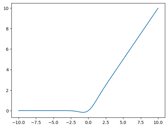
The most well-known variant of ReLU commonly used in NLP is the GELU activation function. The formula for GELU is \(f(x) = x \Phi(x)\) where \(\Phi\) is the Cumulative Distribution Function for the Gaussian Distribution.

This sounds relatively complicated - but if we look at a graph, we see that GELU is simply a variant of ReLU where we have a nonzero derivate for \(x < 0\):

gelu = torch.nn.GELU()

gelu_xs = np.arange(-10, 10, 0.01)
gelu_ys = gelu(torch.tensor(gelu_xs))
plt.plot(gelu_xs, gelu_ys)

[<matplotlib.lines.Line2D at 0x7fd48ad875b0>]

The Embedding Layer

The embedding layer is basically just a simple lookup table that can map IDs to high-dimensional, dense vectors:

embedding_layer = nn.Embedding(num_embeddings=10, embedding_dim=3)

print(embedding_layer.weight)

Parameter containing:
tensor([[ 0.3189, -0.4245,  0.3057],
        [-0.7746,  0.0349,  0.3211],
        [ 1.5736, -0.8455, -1.2742],
        [ 2.1228, -1.2347, -0.4879],
        [-1.4181,  0.8963,  2.2181],
        [ 0.5232,  0.3466, -0.1973],
        [-1.0546,  1.2780,  0.1453],
        [ 0.2311,  0.0566,  0.4263],
        [ 0.5750, -0.6417, -2.2064],
        [-0.7508,  2.8140,  0.3598]], requires_grad=True)

Let’s say that we would like to retrieve the embeddings for IDs 3, 2 and 5. Then, we could simply pass the tensor containing these IDs to the embedding layer:

emb_x = torch.tensor([3, 2, 5])

emb_y = embedding_layer(emb_x)
print(emb_y)

tensor([[ 2.1228, -1.2347, -0.4879],
        [ 1.5736, -0.8455, -1.2742],
        [ 0.5232,  0.3466, -0.1973]], grad_fn=<EmbeddingBackward0>)

As you can see the output contains the rows 3, 2 and 5 from the lookup table.

Note that the lookup table is a learnable parameter:

for name, param in embedding_layer.named_parameters():
    print(name, param)

weight Parameter containing:
tensor([[ 0.3189, -0.4245,  0.3057],
        [-0.7746,  0.0349,  0.3211],
        [ 1.5736, -0.8455, -1.2742],
        [ 2.1228, -1.2347, -0.4879],
        [-1.4181,  0.8963,  2.2181],
        [ 0.5232,  0.3466, -0.1973],
        [-1.0546,  1.2780,  0.1453],
        [ 0.2311,  0.0566,  0.4263],
        [ 0.5750, -0.6417, -2.2064],
        [-0.7508,  2.8140,  0.3598]], requires_grad=True)

Embeddings are extremely useful in LLMs because they allow us to map discrete units (like words or word positions) to high-dimensional, continuous vectors such that the vectors can be learned by the LLM. For example, we could create word embeddings in such a way that semantically similar words result in embeddings that are spatially close to each other. We could then pass these word embeddings to other layers that would learn further features.

Dropout

As we already explained in the chapter on computational graphs, one of the biggest challenges when training neural networks is to avoid overfitting. We briefly talked about a few methods that can be used to accomplish this - however, we haven’t mentioned one of the most important methods known as dropout.

The idea is to randomly drop some neurons during training to prevent them from becoming too dependent on other specific neurons. This way, we force them to learn robust features.

Technically speaking, the dropout layer randomly zeroes some of the elements of the input tensor using sampling from a Bernoulli distribution with probability p. Furthermore, the outputs are normalized via scaling by a factor of 1/(1-p).

Let’s have a look at an example:

dropout_layer = nn.Dropout(p=0.5)

drop_x = torch.randn(5)
print(drop_x)

tensor([ 0.8172,  0.7596,  0.7343, -0.6708,  2.7421])

drop_y = dropout_layer(drop_x)
print(drop_y)

tensor([1.6344, 1.5191, 1.4687, -0.0000, 0.0000])

drop_X = torch.randn(3, 5)
print(drop_X)

tensor([[ 1.5815, -0.1981,  0.9554, -1.0902,  2.5952],
        [ 2.7504,  0.6488,  0.4496,  0.3220, -1.0503],
        [ 0.0274, -0.7916, -0.5601, -0.9977, -0.9444]])

drop_Y = dropout_layer(X)
print(drop_Y)

tensor([[0.4607, 0.0000, -0.0000],
        [-0.0000, 0.0000, 0.0000]])

Note that the dropout layer only drops neurons during training:

print(dropout_layer.training)

True

If we set the dropout layer to evaluation mode using the eval() function, we will see that it no longer drops neurons:

dropout_layer.eval()
print(dropout_layer.training)

False

print(dropout_layer(x))

tensor([0.3367, 0.1288, 0.2345])

If we want to set it back to training mode, we can use the train() function:

dropout_layer.train()
print(dropout_layer.training)

True

print(dropout_layer(x))

tensor([0.0000, 0.2576, 0.4689])

Note that the train() function doesn’t actually do any training, it only sets a layer or a model to training mode.

A common source of bugs when training models is forgetting to set the model to training mode during training or to evaluation mode during evaluation, so be mindful of that.

Layer Normalization

Another important concept for stabilizing training is called layer normalization.

This technique normalizes inputs across features of individual samples in a batch. The idea behind this is to ensure that each input to the next layer has a mean of zero and a variance of one.

To accomplish this, we compute the mean and the variance across features for each sample and then normalize them.

Consider the following tensor:

X = torch.randn(batch_dim, d_in)
print(X)

tensor([[-0.7357, -0.9648, -1.6645],
        [ 0.2046,  0.7237,  0.1275]])

Let’s compute the mean and the variance of that tensor for every feature:

mean = X.mean(dim=-1, keepdim=True)
print(mean)

tensor([[-1.1217],
        [ 0.3519]])

var = X.var(dim=-1, keepdim=True)
print(var)

tensor([[0.2341],
        [0.1051]])

Note that mean contains the mean for every sample in the batch and var contains the variance for every sample in the batch.

We can now normalize the tensor:

X_norm = (X - mean) / torch.sqrt(var)
print(X_norm)

tensor([[ 0.7977,  0.3242, -1.1219],
        [-0.4544,  1.1465, -0.6921]])

If we recompute the mean and the variance of the new tensor, we will find that the mean is now zero and the variance is one for every sample:

X_norm.mean(dim=-1, keepdim=True)

tensor([[    -0.0000],
        [     0.0000]])

X_norm.var(dim=-1, keepdim=True)

tensor([[1.0000],
        [1.0000]])

Commonly, we also scale and shift each normalized feature using learnable parameters scale and shift. If we were to implement a full LayerNorm layer from scratch, it would look as follows:

class LayerNorm(nn.Module):
    def __init__(self, emb_dim):
        super().__init__()
        self.eps = 1e-5
        self.scale = nn.Parameter(torch.ones(emb_dim))
        self.shift = nn.Parameter(torch.zeros(emb_dim))

    def forward(self, x):
        mean = x.mean(dim=-1, keepdim=True)
        var = x.var(dim=-1, keepdim=True, unbiased=False)
        norm_x = (x - mean) / torch.sqrt(var + self.eps)
        return self.scale * norm_x + self.shift 

layer_norm = LayerNorm(d_in)
print(layer_norm(X))

tensor([[ 0.9770,  0.3970, -1.3740],
        [-0.5565,  1.4041, -0.8476]], grad_fn=<AddBackward0>)

Let’s compare our manual layer to the builtin nn.LayerNorm layer to see if our calculations match:

layer_norm_torch = nn.LayerNorm(d_in)
print(layer_norm_torch(X))

tensor([[ 0.9770,  0.3970, -1.3740],
        [-0.5565,  1.4041, -0.8476]], grad_fn=<NativeLayerNormBackward0>)